Blog
Field notes from my Excel work
Most of what I write here started as a problem I hit on a real project — usually at 11pm, usually when something was due in the morning. I write each post after I've fixed the thing, while the lessons are still fresh.
Nehan PatelAuthor
I write every post on Excel Translator. Ten years of spreadsheet work across HR, finance, and engineering teams in three countries. I post when I have something useful to say — about once every two weeks.
2026-04-22 · Translation
Why your German workbook says #NV and not #N/A
Microsoft localizes a handful of error values too — #NV in German, #N/D in Italian, #NV in Polish. The values are interchangeable when the file is opened in another locale, but if you're parsing a CSV export, your script needs to know about both forms.
Read more →
2026-04-08 · Performance
The hidden cost of OFFSET in a 100k-row sheet
OFFSET is volatile — it recalculates on every change anywhere in the workbook. Replacing two OFFSET-based dynamic ranges with structured Table references took a real customer's recalc time from 11 seconds to 0.3.
Read more →
2026-03-24 · Dynamic arrays
SCAN is the running-total function you didn't know you needed
Cumulative sums used to require dragging a =SUM($B$2:B2) formula down a column. With SCAN(0, B2:B100, LAMBDA(a,b, a+b)) you write it once, in one cell, and it spills.
Read more →
2026-03-10 · Pitfalls
The VLOOKUP bug that hides until someone inserts a column
Hardcoded column indices are time bombs. Three real-world examples of how a colleague's "harmless" column insert broke a forecast model — and the one-line XLOOKUP rewrite that prevents it forever.
Read more →
2026-02-26 · LAMBDA
Three custom LAMBDAs every workbook should have
EXTRACT.NUMBERS, NORMALIZE, SAFE.DIV — small, reusable, and immediately useful. Define once in Name Manager, call everywhere.
Read more →
2026-02-12 · Translation
CELL("address") — the argument that doesn't auto-translate
Excel translates the function name when a workbook crosses locales, but not the literal text inside the formula. Here's why =ZELLE("Adresse", A1) stops working when opened in English — and the safer pattern that survives.
See the args reference →
2026-01-28 · Debugging
Why my XLOOKUP returned the wrong value (a 30-minute debug story)
I once spent half an hour staring at an XLOOKUP that kept returning #N/A for values I could see right there in the lookup column. The culprit wasn't the formula — it was a single trailing space hiding in the data.
Read more →
2026-01-15 · Productivity
5 Excel keyboard shortcuts I use 50 times a day
If you use Excel daily and don't know Ctrl+Shift+Arrow, Alt+=, F4, Ctrl+;, and Ctrl+T — these five will give you back ten minutes a day, every day, forever.
Read more →
Featured post
Why your German workbook says #NV and not #N/A
Published 2026-04-22 by Nehan Patel · 5 min read
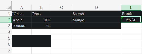
The first time I saw #NV in a German Excel file, I thought it was a typo. I had inherited a pricing model from a colleague who used a German Excel installation, and half the cells were showing this error code I'd never seen before. Five minutes of Googling later: it wasn't a typo, it was just the German localization of #N/A. Microsoft localizes a small set of error values alongside function names. Here are the ones I see most often:
| English | German | Italian | Polish |
|---|
| #N/A | #NV | #N/D | #N/D! |
| #NULL! | #NULL! | #VUOTO! | #ZERO! |
| #NUM! | #ZAHL! | #NUM! | #LICZBA! |
| #REF! | #BEZUG! | #RIF! | #ADR! |
In the workbook itself, this almost never matters — Excel converts the displayed error value to the local form when you open the file. Where it bites is in downstream tooling: a Python script that calls pandas.read_excel() on a German file gets "#NV" back as a string, not NaN. Your filter df[df.col != "#N/A"] silently keeps the bad rows.
The fix is simple but easy to forget: when reading localized Excel files, normalize all the error variants to a single canonical form before any analysis. Or — better — convert them to actual NaN at import time.
// Python example
ERROR_VALUES = {"#N/A","#NV","#N/D","#REF!","#BEZUG!","#RIF!","#NULL!","#VUOTO!","#ZAHL!","#NUM!","#LICZBA!","#WERT!","#VALUE!","#VALOR!","#NOMBRE?","#NAME?","#NOM?","#NOME?","#DIV/0!","#NAZWA?"}
df = df.replace(list(ERROR_VALUES), pd.NA)
Inside Excel itself, prefer formulas that produce a specific friendly fallback over ones that error out. =XLOOKUP(A2, names, scores, "Not found") is locale-proof; =IFERROR(VLOOKUP(A2, t, 3, 0), "Not found") is too. Both ship a string instead of a localized error code, and downstream tools never have to know.
Featured post
The hidden cost of OFFSET in a 100k-row sheet
Published 2026-04-08 by Nehan Patel · 4 min read
I once spent two days investigating why a client's financial model felt sluggish — every cell edit caused a 9-second pause. The model was about 100,000 rows and the team blamed it on hardware. I found the real culprit by accident: 47 OFFSET-based dynamic named ranges. Volatile functions like NOW, TODAY, RAND, OFFSET, INDIRECT, and CELL with certain args recalculate every time anything in the workbook changes. One OFFSET in a 5-row spreadsheet is invisible. Forty-seven of them in a 100,000-row model is a multi-second pause every time someone types a number.
The trap: OFFSET shows up most often in dynamic named ranges, the technique people learned to make ranges auto-extend before Excel had Tables.
// The classic dynamic-range definition (volatile)
SalesRange = OFFSET(Sheet1!$B$2, 0, 0, COUNTA(Sheet1!$B:$B)-1, 1)
Modern replacement: convert the data into an Excel Table (Ctrl+T) and reference it as Sales[Amount]. Tables auto-extend as you add rows, and the reference is non-volatile. Recalc time on the customer file mentioned in the title dropped from ~11s to ~0.3s after this single change.
If you must keep a dynamic range without a Table — for example, in a workbook that has to open in older Excel — the non-volatile alternative uses INDEX:
SalesRange = $B$2:INDEX($B:$B, COUNTA($B:$B))
INDEX is not volatile, even when used to construct a range. Same effect, no recalc tax.
Featured post
SCAN is the running-total function you didn't know you needed
Published 2026-03-24 by Nehan Patel · 6 min read
For ten years, every time I needed a running total in Excel I did the same thing: typed =SUM($B$2:B2) in cell C2, then dragged the fill handle down a thousand rows. It worked. But it always felt clumsy — drag too short and you miss rows; drag too far and you waste calc cycles on empty cells; insert a row in the middle and the formula doesn't always refit.
Then I learned about SCAN, and I haven't dragged a running total since.
The old way: drag-fill SUM
// In C2, drag down to C1000:
=SUM($B$2:B2)
This works because of the mixed reference: $B$2 stays anchored, B2 grows with each row. So in C5 the formula becomes =SUM($B$2:B5) — exactly what we want. But every cell holds its own formula, every cell recalculates independently, and the whole pattern lives or dies by whether someone remembers to extend the drag when new data arrives.
The new way: one SCAN formula, everywhere
Type this once, in C2:
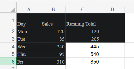
=SCAN(0, B2:B100, LAMBDA(a, b, a + b))
That's it. The result spills down through C2:C100 automatically — one formula, one cell, every running total is correct. If B11 changes, only C11 onwards recalculates.
Reading the formula left to right: SCAN takes three arguments. The first is the initial value (zero — we start the running total at zero). The second is the array to walk through (the daily values in B2:B100). The third is a LAMBDA accumulator function — for each item b, combine it with the running total a. In our case, addition: a + b.
What else SCAN can do
Once you see the pattern, you'll find uses everywhere. Running totals are the obvious one, but SCAN handles any "carry-forward" calculation:
Running maximum (rolling high-water mark)
=SCAN(0, B2:B100, LAMBDA(a, b, MAX(a, b)))
For tracking the highest stock price seen so far, the longest streak, the personal best in a fitness log.
Compounding interest
=SCAN(1000, returns, LAMBDA(a, r, a * (1 + r)))
Starting with ₹1,000, apply each return as a multiplier. The third row of the spilled output is your balance after three periods.
Inventory ledger (with restocks)
=SCAN(0, B2:B100, LAMBDA(a, change, MAX(0, a + change)))
Adds positive changes (restock), subtracts negative ones (sales), but never goes below zero.
When to keep the old SUM approach
I haven't completely retired the dragged SUM pattern. Two cases where it's still the right choice:
- Excel 2019 or older. SCAN and LAMBDA require Excel 365 or 2021+. If your workbook needs to open on older Excel, stick with
=SUM($B$2:B2).
- You need different starting points per group. If C is broken into groups (orders by region, classes by date) and each group should reset to zero, a vanilla
SCAN won't reset — you'd need extra logic. The dragged SUMIFS approach is sometimes simpler.
The bigger pattern
Once you've used SCAN, look at the rest of the LAMBDA helper family: MAP (transform each value), REDUCE (combine to a single value), BYROW / BYCOL (apply across rows or columns). They turn Excel's formula language into something close to a real programming language. Once you start thinking in arrays-and-lambdas instead of single-cell-and-drag, you stop writing the same formula a thousand times.
If you do one Excel upgrade this quarter, it's this. Replace one dragged-down formula with a single SCAN, see how much cleaner the worksheet becomes, and you'll be looking for excuses to use it.
Featured post
The VLOOKUP bug that hides until someone inserts a column
Published 2026-03-10 by Nehan Patel · 7 min read
I want to tell you about a bug that almost cost a sales team their quarterly demo. The setup: a pricing dashboard that pulled product details from a master sheet via VLOOKUP. It had worked perfectly for six months. Then someone — trying to be helpful — inserted a "Region" column into the master sheet. The dashboard kept loading, no error appeared, and the prices on every row silently became product names.
Nobody noticed for three days, because the dashboard didn't crash. It just lied.
How VLOOKUP fails silently
The dashboard formula was the textbook VLOOKUP pattern:
=VLOOKUP(A2, Products, 4, FALSE)
"Look up the product ID in A2 within the Products table, return the value from column 4." When the table was [ID, Name, SKU, Price], column 4 was Price. Perfect.
Then someone inserted "Region" between ID and Name. The table became [ID, Region, Name, SKU, Price]. Column 4 was now SKU. Column 5 was the price. The VLOOKUP happily returned column 4 — the SKU codes — and rendered them in the price column of the dashboard. The dashboard's Price column now displayed values like "PRD-X-9821" instead of "₹12,500", and because everyone scanned for visual patterns rather than reading every value, the issue stayed invisible.
Why this is a category of bug, not just a one-time mistake
The deeper problem is that VLOOKUP identifies columns by position number — and a position number is a fragile reference. Every time someone:
- Inserts a new column anywhere to the left of your target
- Reorders columns for "readability"
- Hides a column thinking it's unused
- Copies the lookup table to a new sheet with slightly different structure
...your VLOOKUP can either error or, much worse, silently return the wrong column. There is no warning. The formula doesn't know you meant "Price" — it only knows you said "the fourth column from the left."
The fix: XLOOKUP by named range
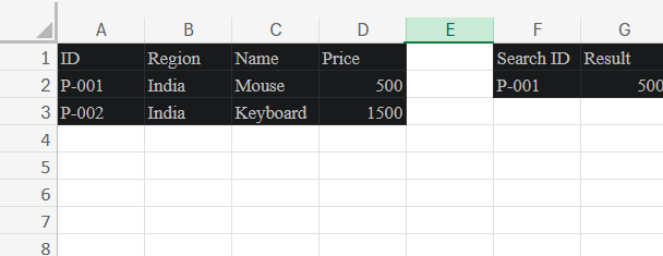
The same lookup, written with XLOOKUP:
=XLOOKUP(A2, Products[ID], Products[Price], "Not found")
This is bullet-proof in the way VLOOKUP isn't:
- It references
Products[ID] and Products[Price] by name, not by position. Insert any number of columns between them — the formula still finds the right ones.
- The "Not found" fallback is built in. No more
=IFERROR(VLOOKUP(...), "Not found") wrapper.
- You can search bottom-up, exact match, approximate, wildcard — XLOOKUP has flags for all of it.
VLOOKUP has approximate-match-by-default which is the source of about half its remaining bug reports.
The migration playbook
If you have a workbook full of VLOOKUPs and you want to upgrade safely, here's the order I follow:
- Convert the lookup tables to Excel Tables (Ctrl+T). This gives you the
Products[Column] syntax that XLOOKUP loves. It also makes ranges auto-extend when new rows arrive.
- Find every
VLOOKUP with Ctrl+F → "VLOOKUP" → "Find All". Excel gives you a list with cell references — work through them top to bottom.
- For each one, replace the formula. The mechanical translation is:
=VLOOKUP(K, Tbl, n, 0) becomes =XLOOKUP(K, Tbl[lookup_col], Tbl[return_col], "Not found").
- Test with a few known values before you celebrate. The numbers should match what
VLOOKUP returned — if they don't, your VLOOKUP was probably already wrong.
- Document the migration in a worksheet or sticky note: which formulas were swapped, which weren't, why. Future-you will thank present-you.
Keep VLOOKUP for…
Honest disclosure: VLOOKUP isn't dead. Two scenarios where I still use it:
- Workbooks shared with people on Excel 2019 or older. XLOOKUP doesn't exist there.
VLOOKUP remains the lowest common denominator.
- Quick one-off lookups where you'll delete the formula in five minutes. The migration tax isn't worth paying.
For everything else — anything that lives in a workbook longer than a week, anything someone else might edit, anything that drives a decision — XLOOKUP wins. And after the column-insert bug I described above, I haven't shipped a new VLOOKUP to a client in over a year.
Featured post
Three custom LAMBDAs every workbook should have
Published 2026-02-26 by Nehan Patel · 8 min read
The first time I wrote a LAMBDA, I felt the same shift in posture I felt when I first wrote a function in JavaScript. Suddenly Excel wasn't a place where I copy-pasted formulas — it was a place where I could define a piece of logic once, name it, and call it like a built-in.
Three years in, I have about a dozen LAMBDAs that live in every serious workbook I build. Three of them earn their keep more than the rest. If you're new to LAMBDA, start with these.
1. EXTRACT.NUMBERS — pull digits out of messy text
Every dataset I've ever inherited has had at least one column where someone typed prices, quantities, or IDs as messy text: "Order #1-2456", "₹ 12,500.00", "PRD-X-9821". Pulling the numeric part out used to take three nested formulas. With LAMBDA, it's one named call.
Define this once via Formulas → Name Manager → New:
Name:    EXTRACT.NUMBERS
Refers to:
=LAMBDA(text,
  VALUE(
    TEXTJOIN("", TRUE,
      IFERROR(MID(text, SEQUENCE(LEN(text)), 1) * 1, "")
    )
  )
)
Now anywhere in the workbook:
=EXTRACT.NUMBERS("Order #1-2456")     // returns 12456
=EXTRACT.NUMBERS("₹ 12,500.00")        // returns 1250000
=EXTRACT.NUMBERS(A2)                   // works on any cell
How it works: SEQUENCE(LEN(text)) generates positions 1, 2, 3... up to the length. MID pulls out one character at each position. Multiplying by 1 forces a number conversion — letters fail with an error, digits become themselves. IFERROR turns failures into empty strings. TEXTJOIN sticks the survivors back together. VALUE wraps the result as a real number.
It's not perfect — it can't handle decimals or negative signs perfectly — but for the 90% case (extract digits from text), it's a one-line fix that would otherwise be twenty.
2. NORMALIZE — clean text columns before lookups
Half the lookup bugs I've debugged came down to the same root cause: trailing whitespace, mixed case, or non-breaking spaces in the lookup column. So I built a normalize function that I run on every text column before doing any matching:
Name:    NORMALIZE
Refers to:
=LAMBDA(text,
  TRIM(
    CLEAN(
      LOWER(text)
    )
  )
)
Three things happen: LOWER drops case sensitivity. CLEAN strips non-printable characters (the kind that sneak in from CSV exports). TRIM removes leading, trailing, and duplicate internal whitespace. Run it on both sides of a lookup:
=XLOOKUP(NORMALIZE(A2), NORMALIZE(names), emails, "Not found")
I now run NORMALIZE habitually whenever a lookup misbehaves. About 80% of the time, the problem disappears.
3. SAFE.DIV — divide without #DIV/0!
The simplest of the three. Division by zero crashes calculations, breaks dashboards, and generally causes more #DIV/0! errors than it should:
Name:    SAFE.DIV
Refers to:
=LAMBDA(numerator, denominator,
  IF(denominator = 0, 0, numerator / denominator)
)
Now every division I write is safe by default:
=SAFE.DIV(B2, C2)              // returns 0 if C2 is 0
=SAFE.DIV(SUM(sales), SUM(units))   // returns 0 if no units
You can extend it to return a custom fallback (like "—" for dashboards), but the zero default works for most accounting/finance contexts.
How to install these in your workbook
LAMBDAs defined via Name Manager only exist in that workbook. To use the same three LAMBDAs across many workbooks:
- Save them in a Personal Macro Workbook style template. Create a "starter.xlsx" with these three LAMBDAs already defined; copy it as the basis for new projects.
- Or use Office 365's LAMBDA library (rolling out to enterprise customers in 2026) — once enabled, you define a LAMBDA once and call it across every workbook tied to your account.
- Or paste the formulas in directly as comments at the top of new workbooks; copy them into Name Manager when needed.
What other LAMBDAs are worth the time?
The three above are my non-negotiables. Honourable mentions: DATEDIF.YM (years and months between dates, formatted "5y 3m"), WEEKDAYS.BETWEEN (count working days respecting custom weekends), ARRAY.UNIQUE.SORTED (one-shot dedupe + sort). If there's interest, I'll write those up next.
The bigger lesson: LAMBDA isn't about clever formulas, it's about not repeating yourself. Anything you find yourself typing for the third time is a candidate. Name it, save it, and stop typing it.
Featured post
Why my XLOOKUP returned the wrong value — a 30-minute debug story
Published 2026-01-28 by Nehan Patel · 6 min read
One Tuesday afternoon I lost half an hour to an XLOOKUP that simply refused to find a value I could see right there in the lookup column. The formula looked fine. The data looked fine. The result was #N/A.
Here's what happened, what I tried, and the embarrassingly small fix that ended it.
The setup
I was building a contact lookup utility for a small CRM. Names in column A, emails in column B. A search box in D2. The result formula:
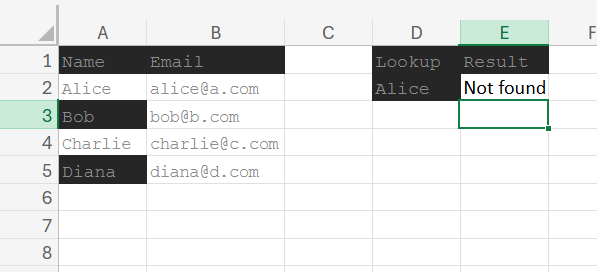
=XLOOKUP(D2, A2:A8, B2:B8, "Not found")
I typed "Alice" into D2. The formula returned #N/A. But Alice was right there in cell A2.
What I tried first (all dead ends)
Was the range wrong? I checked. A2:A8 covered the names. B2:B8 covered the emails. Same number of rows. Fine.
Was the search value blank? =LEN(D2) returned 5. "Alice" — the letters were there. Fine.
Was case sensitivity the issue? I tried =XLOOKUP(LOWER(D2), LOWER(A2:A8), B2:B8, "Not found"). Still #N/A. Excel's XLOOKUP isn't case-sensitive by default anyway, but worth checking.
Did XMATCH see it? =XMATCH(D2, A2:A8) also returned #N/A. So the problem was upstream of the lookup — the values genuinely weren't matching.
Was the data being treated as text? Both sides were text. No type mismatch.
At this point I almost gave up and rebuilt the data. Then I noticed something.
The clue
I clicked into A2. The cell showed "Alice". But the formula bar showed... a tiny gap after the "e". I clicked at the end of "Alice" with the keyboard. The cursor sat one position to the right of where I expected.
A trailing space. The cell didn't contain "Alice". It contained "Alice " — five letters and a single space.
"Alice" (what I typed in D2) is not equal to "Alice " (what was in A2). XLOOKUP, doing its job correctly, found no match.
Where the trailing space came from
The names had been pasted in from an Excel file someone exported from their email client. Most CRM exports preserve trailing spaces from the original data — they're invisible visually but they break every text comparison.
If you've ever wondered why your lookups work for the first ten names you test and fail for an obscure eleventh, this is the answer about three times out of four. You typed the eleventh name; you didn't paste it. Trailing space mismatch.
The fix
TRIM on both sides:
=XLOOKUP(TRIM(D2), TRIM(A2:A8), B2:B8, "Not found")
TRIM removes leading/trailing whitespace and collapses repeated internal spaces to a single space. Apply it to the lookup value and the lookup array, and trailing-space mismatches stop existing.
That fixed it. The whole rabbit hole was 30 minutes; the actual fix was four characters of typing.
What I do now, by default
Since this incident I treat any text lookup with suspicion until I've trimmed both sides. My standard pattern is:
=XLOOKUP(TRIM(D2), TRIM(names), values, "Not found")
If I expect non-printable characters too (anything imported from web/HTML), I add CLEAN:
=XLOOKUP(TRIM(CLEAN(D2)), TRIM(CLEAN(names)), values, "Not found")
For frequently-used lookups I wrap this in a NORMALIZE LAMBDA (see my LAMBDA post above). After that, lookup bugs basically stop happening for me.
How to spot the trailing space yourself
Three quick checks any time a lookup fails:
- Click the cell. End key. Compare cursor position with where you expected text to end. Off by one? Trailing space.
=LEN(A2) — does the length match the visible character count?=A2 = D2 — straight comparison. FALSE when they look identical means hidden whitespace.
Two minutes with these three checks would have saved my afternoon. Now you know — so it'll save yours.
Featured post
5 Excel keyboard shortcuts I use 50 times a day
Published 2026-01-15 by Nehan Patel · 5 min read
If you spend more than an hour a day in Excel, the difference between knowing five shortcuts and knowing zero is roughly ten minutes per day. Over a working year, that's about 40 hours — a full week. These are the five I'd defend hardest if someone tried to take Excel shortcuts away from me.
I've ordered them by how often I press them. The first one is essentially muscle memory at this point.
1. Ctrl + Shift + Arrow — select to the edge of data
This is the king. Click anywhere in a column with data, press Ctrl+Shift+↓, and Excel selects every cell from the cursor to the last non-empty cell in that column. → selects across columns. The combinations stack.
The version most people learn — Ctrl+End — selects all the way to the last used cell of the entire worksheet, which is rarely what you want. Ctrl+Shift+Arrow selects to the edge of the current data block, which is what you actually mean nine times out of ten.
I learned this one after watching a colleague select a 40,000-row column by clicking the header, dragging, scrolling, dragging some more. He took 30 seconds. The shortcut takes half a second.
2. Alt + = — auto-sum
Place the cursor in an empty cell directly below or to the right of a column/row of numbers. Press Alt+=. Excel writes =SUM(...) with the right range pre-filled. Press Enter and you have your total.
It works for entire selections too — select a range with one extra empty row at the bottom and one extra empty column on the right, press Alt+=, and Excel fills in row totals, column totals, and a grand total in one go. This used to take me a minute of typing; now it takes two seconds.
3. F4 — toggle $ on the reference under the cursor
While editing a formula, place the cursor inside a cell reference (like A1). Press F4. Excel cycles: A1 → $A$1 → A$1 → $A1 → A1.
This replaces the painful "type the dollar signs by hand" workflow. If you've ever typed =$A$1 manually, you know how many wrong-finger errors that produces. F4 is correct every time.
On Mac the equivalent is ⌘+T.
4. Ctrl + ; — insert today's date as a static value
Type today's date into a cell without using the volatile =TODAY() formula (which recalculates every time the workbook changes, and on every reopen). Ctrl+; drops in the current date as a literal value that doesn't move.
The variant Ctrl+Shift+: drops in the current time. I use the date one constantly when logging entries — purchase dates, status updates, daily summaries — anything where I want today's date but don't want it to drift.
5. Ctrl + T — convert range to a Table
This isn't really a navigation shortcut — it's a structural transform. Place the cursor in any data range (one cell is enough), press Ctrl+T, confirm the range, and Excel turns the data into a Table.
Why is that worth a shortcut? Tables auto-extend when you add rows. Formulas that reference a Table column (SalesTable[Amount]) auto-include the new rows. Filters and sorts work better. Charts based on the Table grow with the data. And the structured-reference syntax reads like English — SalesTable[@Amount] * 1.18 is much clearer than F2 * 1.18.
For data that lives more than 10 minutes, I convert to a Table by reflex.
Bonus shortcuts that nearly made the list
- Ctrl + 1 — open the Format Cells dialog. The fastest way to set number formats, borders, alignment.
- Ctrl + D / Ctrl + R — fill down / fill right. Replaces the click-and-drag-the-corner workflow.
- Ctrl + ` (the backtick) — toggle showing all formulas instead of values. Lifesaver when auditing a workbook you didn't build.
- F2 — edit the current cell without using the mouse to click the formula bar.
How to actually learn shortcuts
You don't memorise five shortcuts by reading a list. You learn them by banning yourself from the slow alternative for one week. Whatever you usually do with the mouse, force yourself to use the keyboard for that week. After a week, the shortcuts are in your hands and you stop thinking about them.
Try Ctrl+Shift+Arrow for one week. After that, the others fall in naturally — once you've banned the mouse for selection, you start banning it for everything else too.
Nehan PatelAuthor
I post about once every two weeks — usually after I've fixed something interesting on a client project. If a post here saved you time, the best thanks is to tell me what to write about next.